Billy Wayne McCann, Ph.D.

avo_ibo

GitHub · BSD 3-Clause · 2025–2026

avo_ibo brings Intrinsic Bond Orbitals directly into Avogadro 2. It uses Psi4 for SCF and wavefunction generation, then performs post-SCF orbital construction inside the plugin as a complete implementation of the IAO/2014 algorithm.

The result is a streamlined workflow: compute, localize, and inspect orbitals without switching tools. Occupied IBOs, valence-virtual IBOs, and analysis outputs are generated in one in-process pipeline and shown directly in Avogadro’s Molecular Orbitals panel.

Why this matters: IBO generation is integrated into the same editor used to build and interpret structures, reducing tool switching and improving reproducibility for teaching and research.

Workflow in 3 Steps

1. Run Electronic Structure

Compute the wavefunction with Psi4 (HF or DFT).

2. Build and Localize IBOs

The plugin performs IAO construction, PM localization, degeneracy resolution, and valence-virtual generation.

3. Inspect in Avogadro

Orbitals and analysis data appear in the Molecular Orbitals panel for interactive interpretation.

What You Can Do With It

Compute IBOs for neutral closed-shell systems using HF or DFT, from small molecules to representative transition states
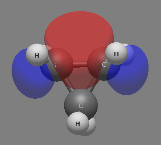
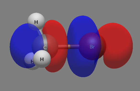
Inspect orbital isosurfaces in Avogadro with direct toggling and interactive rotation
Analyze occupied IBOs (σ, π, lone pairs, core) and valence-virtual IBOs (σ*, π*) in one workflow
Use the analysis table for assignment and interpretation (occupancy, energy, bond type, composition, hybridization)
Run headless workflows with python -m avogadro_ibo molecule.xyz for scripts and batch jobs
Adjust basis sets and methods (for example, cc-pVDZ, cc-pVTZ, and B3LYP) through plugin options

Use Cases

Teach bonding models with computed orbitals rather than schematic sketches
Prepare publication figures that connect orbital shape to mechanistic interpretation
Perform rapid orbital inspection during exploratory computational workflows

Orbital Visualizations

Cyclopropane C–C σ bond IBO — Cyclopropane C–C σ bond showing bent-bond character. Electron density is displaced from the internuclear axis and curves outward, consistent with this molecule’s unusual reactivity.

Methyl bromide C–Br σ* LUMO IBO — Methyl bromide C–Br σ* LUMO, the anti-bonding orbital central to S_N2 discussion, shown as a computed orbital with the expected nodal plane between carbon and bromine.

Quick Start

Requires pixi.

git clone https://github.com/exergonic/avo_ibo.git
cd avo_ibo
pixi install
pixi run python -m pip install -e .

Standalone CLI

pixi run python -m avogadro_ibo molecule.xyz

Reads an XYZ file, runs the full IBO pipeline, and writes results to calcs/last/ (ibo.molden, canonical.molden, ibos.txt, psi4.log). Supports neutral singlets only.

Avogadro 2 plugin

Create a symlink so Avogadro discovers the plugin:
(requires Administrator or Developer Mode)

New-Item -ItemType SymbolicLink -Path "$env:LOCALAPPDATA\OpenChemistry\Avogadro\plugins\avo_ibo" `
  -Target "C:\path\to\avo_ibo"

Then in Avogadro: Extensions → Intrinsic Bond Orbitals → Compute IBOs. Computed IBOs appear in the Molecular Orbitals panel, where double-click toggles orbital isosurfaces.

Tests

pixi run test

Seven CLI integration tests against water, methane, ethene, and ammonia validate IAO counts, Molden structure, occupancy partitioning, and per-molecule orbital patterns.

How It Works (At a Glance)

Starting from an input geometry, the plugin requests a wavefunction from Psi4, then performs all post-SCF orbital construction internally. The implementation includes IAO basis construction, Pipek–Mezey localization, on-atom degeneracy resolution, and SVD-based valence-virtual IBO generation.

This yields chemically intuitive orbitals that are immediately available for visualization and assignment. The full pipeline runs in a single Python process with JSON-based Avogadro communication and detailed debug logging for reproducibility and troubleshooting.

A full mathematical derivation of every step is in mathematics.md for those who want the equations.

For the Professionals

The sections below describe the plugin’s complete IAO/2014 implementation: manual post-Psi4 IAO construction, Pipek–Mezey localization with on-atom degeneracy resolution, SVD-based valence-virtual construction, tested molecules, the donor–acceptor analysis limitation, and build architecture.

Pipeline Overview

Geometry → Psi4 HF/cc-pVDZ → C_occ (occupied MO coefficients)
    ↓
C_IAO, C_IAO_occ = _build_iao_basis(S_full, S12, S_min, C_occ)
    ↓
_localize_ibos(C_IAO_occ)      ← PM p=2 → p=4 warm-start
    ↓
_resolve_on_atom_mixing(C_IAO_occ)  ← Fock diag per same-atom group
    ↓
Valence-virtual: SVD(S_IbVir) → U_val → _localize_ibos(U_val)
    ↓
Combine, sort by energy → Molden output → analysis table

The IAO construction is implemented directly in the plugin and follows Appendix C of the Knizia 2013 paper, matching IboView’s MakeIaoBasisNew. A minimal basis (STO-3G) is projected into the full AO space, and the resulting Intrinsic Atomic Orbitals are symmetrically orthogonalized. These IAOs exactly span the occupied space — every occupied MO can be expressed as a linear combination of IAOs with zero loss.

The Pipek–Mezey localization (p=4, convergence 1e-12, max 2048 iterations) uses a warm-start strategy: first solve with the convex p=2 functional, then refine with p=4. This avoids shallow local minima that can trap a cold p=4 start. The Jacobi sweep algorithm rotates orbital pairs to maximize atomic population concentration, yielding chemically intuitive σ bonds, π bonds, lone pairs, and core orbitals.

On-Atom Degeneracy Resolution

The PM functional depends only on atomic populations, so orbitals that both sit on the same atom with DOM ≈ 1 (e.g. O 2s and the oxygen lone pair in water) can mix arbitrarily without changing the localization measure. After PM, a post-processing step diagonalizes the Fock matrix within each same-atom, high-DOM subspace, restoring the aufbau ordering (s-rich lowest, p-rich highest).

Tested Molecules (HF/cc-pVDZ)

Molecule	n_min	Occupied IBOs	Virtual IBOs
Water	7	O(Core), O 2s (s-rich LP), O 2p (pure LP), 2× O–H σ	2× O–H σ*
Methane	9	C(Core), 4× C–H σ (sp³)	4× C–H σ*
Ethene	14	2× C(Core), 4× C–H σ, C–C σ, C–C π	C–C π, 4× C–H σ, C–C σ*
Ammonia	8	N(Core), 3× N–H σ, N(LP) sp³	3× N–H σ*
Formaldehyde	12	O(Core), C(Core), C–O σ, 2× C–H σ, C–O π, O(LP s-rich), O(LP pure p)	C–O π, 2× C–H σ, C–O σ*

A Note on Donor–Acceptor Analysis

Unlike NBOs, the IAO basis exactly spans the occupied space — it is a lossless representation of the occupied MOs. This exactness is a mathematical identity (proved in the mathematics document), not a numerical approximation. As a consequence, the occupied–virtual off-diagonal block of the Fock matrix in the IAO basis is identically zero, making NBO-style E(2) donor–acceptor analysis structurally impossible. This is a feature of the IBO design: IAOs give clean, chemically intuitive orbital shapes for visualization, but they cannot report hyperconjugation energies.

Architecture

The plugin is structured as a standard Avogadro 2 Pixi Python script plugin. It uses uv_build and produces a lock file v6 for compatibility with Avogadro’s pixi. All computation runs in-process (single Python process, no subprocess or file-based IPC to Psi4). Psi4 is used for SCF/wavefunction generation, while the downstream IAO/2014 construction and localization stack is implemented manually in the plugin, with careful logging redirect to avoid stderr contamination of the JSON output that Avogadro parses.

For implementers, a detailed tutorial on building Avogadro 2 Pixi plugins is in tutorial.md (758 lines), covering architecture, algorithm walkthrough, and practical development pitfalls.